Lagrangian Coherent Structures: T106 Low Pressure Turbine Blade

The backward FTLE for T106 LP turbine blade

 

Forward FTLE T106 LP turbine blade

Lagrangian Coherent Structures: Double Gyre and Forced Duffing Equation

Following is the depiction of double gyre with integration time increasing from T=0 to T=15. It could be observed that the number of ridges increase with an increase in integration time T.

 

The next video depicts Forward Finite Time Lyapunov Exponents with a fixed integration time T while the time t in the formula of double gyre is increasing.

 

The last video is the Forward Finite Time Lyapunov Exponents of a forces Duffing equation, with the integration time T=15 and time t increasing from 0 to 10.

MATLAB code for two dimensional Lagrangian Coherent Structure (LCS)

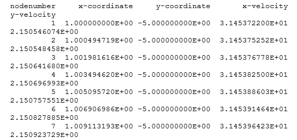
The code was written with the help of Shadden et al.*  To utilize this code one needs to input files consisting information regarding node location and respective x and y velocities at required time steps. Files generated during a CFD simulation using software like ANSYS FLUENT can also be used. Following figure shows the required format for input data files.

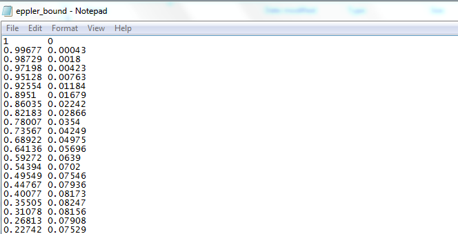
I will use the example from Lipinski et al.**, an eppler 387 airfoil is considered at angle of attach 4 degrees and Re. 60,000 to run the code.

The boundary nodes of the airfoil are saved inside a text file named eppler_bound.txt. The format of this text file is as follows.

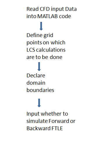
The structure of MATLAB code used is as under,

Velocity data is stored in files numbered, every file consists of data at timestep dt from the previous file. As the time step is small the code pick up a file after df files.

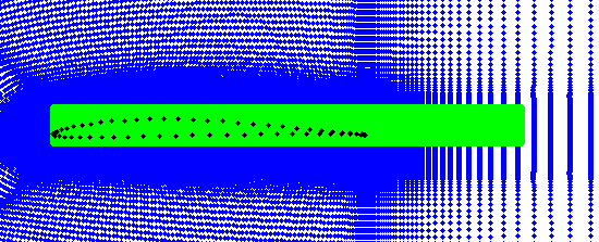
In the figure the blue nodes are the ones imported using data files, while the green nodes are the grid point on which LCS computations are to be performed.

When the code is run it asks user to if forward FTLE or backward FTLE are to be calculated.

From the figure above we can see that the green region inside the airfoil boundary is not required. After the code is run it will ask the user to press 0 if the required nodes are the ones inside the boundary or press 1 if the required nodes are the ones outside the boundary. In this case we will press 1.

 

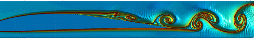
The above figure shows backward FTLE field generated using the above MATLAB code.

Remarks

To get the code email at auwais.ahmed@yahoo.com

The code used Euler scheme for time integration, for better accuracy higher order schemes should be used.

Comments and suggestions are welcome.

References

*Shadden, S., Lekien, F., and Marsden, J., “Definition and Properties of Lagrangian Coherent Structures from Finite-Time LyapunovExponents in Two-Dimensional Aperiodic Flows,” Physica D,Vol. 212, Nos. 3–4, Dec. 2005, pp. 271–304.

** Lipinski, D., Cardwell, B., and Mohseni, K.,”A Lagrangian analysis of a two-dimensional airfoil with vortex shedding”, J. Phys. A: Math. Theor. 41 (2008) 344011 (22pp)

Lagrangian Coherent Structures in Fluid Flows

Study of fluid flow is an important task performed by scientific and engineering community in today’s fast developing world. Such studies find their way in some of the most important applications nowadays. The industries like aerospace, automotive, medical and energy etc expand a huge amount of time and energies in pursuit of proper understanding in this field. With time many computational techniques have been developed to model fluid flows using computers which are becoming more and more powerful with coming time. Today numerical methodologies to simulate phenomena like those occurring in turbomachinery and combustion etc have been developed and are being improved. All these phenomena are very complex and results obtained using these models need interpretation. Several visualization techniques are present that can be used as a tool that can help engineering and scientific researchers in analysis of results. The problem exists in making sense of turbulence that is present in complex flows. Despite the complexity of turbulent flow however these flows are not completely devoid of any structure. In flows there exist certain localized regions which maintain structure. Such localized bounded structures with common topological properties are named as coherent structures. The fact that turbulent flows are not totally chaotic but there is existence of localized coherent structures is important in study of complex fluid flows. One of the examples of such coherent structures is a vortex. These structures are thought to be responsible for the dynamic properties of the flow. The non coherent portion of flow is passive and is advected over the domain by the effect of coherent structures. This means that only the coherent structures can be analyzed to access the general behavior of the flow. Generally the coherent structures are present in a small region of the flow while the larger portion of the flow is non-coherent. However this is not always true. As generally simulating turbulence is computationally expansive only the coherent structures can be simulated to analyze the dynamics of flow.

In the study of dynamical systems a separatrix can be imagined as a manifold attached to fixed points across which there is zero mass flux. Fluid flow is one of the examples of such dynamical system. This gives an opportunity for exploiting this property of such manifolds to elaborate structure in fluid flow and also to detect the presence of coherent structures. In case of problems like fluid flow and many such physical problems the fixed points are not stationary. In fact they can be constantly moving with time. This presents a problem in using traditionally analytical techniques for dynamical systems to find these manifolds in fluid flow. To tackle this problem a technique of Lagrangian Coherent Structures is used to identify these dynamic manifolds in fluid flows. A Lagrangian Coherent Structure is a mobile separatrix with zero mass flux property or with minimum leak. LCS is a material line that is defined as the smooth curves of fluid particles that acts as a transport barrier and is an invariant manifolds. These structures are called Lagrangian because they use a series of time steps defining the motion of fluid particles to calculate instead of the Eulerian approach, that only uses instantaneous time frames. The term coherent structures in the name are used because the LCS delineates the familiar coherent structures associated with the flow. LCS are material lines that have locally maximum attraction or repulsion to the fluid particles.

The property that LCS are material line with maximum local attraction and repulsion can be used to compute them. This technique uses Finite Time Lyapunov Exponents; FTLE would be further discussed in the course of this document. A domain or particles is integrated in time to find the trajectories of particles after a certain finite time. This information is then used to calculate the FTLE field. The rides in the FTLE field depict the manifolds or material lines. For the computation of repelling material lines or stable manifolds the particles are integrated forward in time. In case the computation of unstable manifolds or attracting material lines is desired the particles are integrated backwards in time as the expansion of particles in backward time simulation will represent the attraction of particles in forward time simulation.